Computer vision interview questions and answers

The model hit 97% on the validation set and 61% in the field. The interviewer asked what he thought happened. "Overfitting," the candidate said. "On 200,000 images with heavy augmentation?" It turned out the training photos were all shot in one warehouse under one lighting rig, and the field cameras were in daylight. Not overfitting. Distribution shift — which is a different problem with a different fix.

Computer vision interview questions split neatly into two halves: the mechanics you can be quizzed on, and the data reality that decides whether a model works. This guide covers convolutions and receptive fields, the architectures worth knowing, detection metrics like IoU and mAP, augmentation, and the deployment constraints that come up in every applied loop.

What computer vision interviews actually test

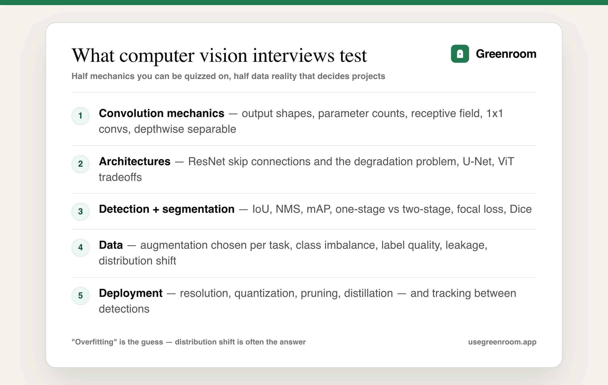
Computer vision interview questions appear in ML engineer, applied scientist, robotics and edge-AI loops. Five bands:

• Convolution mechanics — kernels, stride, padding, output shapes, parameter counts, receptive field.
• Architectures — why ResNet mattered, and what came after.
• Task families — classification, detection, segmentation, and the metrics for each.
• Data — augmentation, class imbalance, labelling quality, distribution shift.
• Deployment — latency, model size, quantization, edge constraints.

Convolution mechanics and the arithmetic you will be asked to do

Expect to compute an output shape on a whiteboard. The formula, worth knowing cold:

def conv_out(in_size, kernel, stride=1, padding=0):
    """Output spatial size for one dimension."""
    return (in_size - kernel + 2 * padding) // stride + 1

def conv_params(k_h, k_w, in_ch, out_ch, bias=True):
    """Learnable parameters in a conv layer."""
    return (k_h * k_w * in_ch + (1 if bias else 0)) * out_ch

# ResNet stem: 224 input, 7x7 kernel, stride 2, padding 3
print(conv_out(224, 7, stride=2, padding=3))        # 112
print(conv_params(3, 3, 64, 128))              # 73856

# Two stacked 3x3 vs one 5x5: same receptive field, fewer params
print(conv_params(3, 3, 64, 64) * 2)          # 73856
print(conv_params(5, 5, 64, 64))               # 102464

Related concepts that come as follow-ups:

• Why convolutions instead of fully connected layers? Parameter sharing (the same kernel slides everywhere), translation equivariance, and locality. A fully connected layer on a 224×224 image has an absurd parameter count and no spatial prior.
• Receptive field — how much of the input one output unit sees. It grows with depth, and this is why stacking two 3×3 convolutions is preferred over one 5×5: the same receptive field, fewer parameters, and an extra non-linearity.
• 1×1 convolutions — they do not look at neighbours, so they exist to mix channels and change channel depth cheaply. Used everywhere in bottleneck blocks.
• Pooling vs strided convolution — both downsample; pooling is parameter-free and fixed, strided convolution is learned. Modern architectures often prefer the latter.
• Depthwise separable convolutions — factorise spatial and channel mixing for a large parameter reduction. The basis of MobileNet and the standard answer to "how would you shrink this model?"

Architectures: what to know and why

You do not need to recite every architecture, but you need the story of why each mattered:

• ResNet — the one to know cold. Skip connections let gradients flow directly backwards, which solved the degradation problem where deeper plain networks performed worse than shallow ones. Say that clearly and you have answered most architecture questions.
• VGG — showed that stacks of small 3×3 kernels work well; mostly of historical interest now, and useful as a contrast.
• Inception — parallel multi-scale kernels in one block, plus 1×1 bottlenecks for efficiency.
• EfficientNet — compound scaling of depth, width and resolution together rather than one at a time.
• Vision Transformers — images as sequences of patches with self-attention. Beat CNNs at scale, but are data-hungry; hybrid and CNN approaches remain strong in limited-data and edge settings, which is an honest nuance worth voicing.
• U-Net — encoder-decoder with skip connections between matching levels, the default for segmentation and widely used in medical imaging and diffusion models.

Also expect transfer learning, which is how most real projects start: take an ImageNet-pretrained backbone, replace the head, freeze early layers and fine-tune later ones. Know why early layers transfer well — they learn generic edges and textures — and when full fine-tuning is worth it, which is when your domain is far from natural images, like X-rays or satellite data.

Object detection: IoU, NMS and mAP

The metrics questions are asked precisely because candidates fudge them. Get these exact:

• IoU (Intersection over Union) — area of overlap divided by area of union between predicted and ground-truth boxes. A prediction usually counts as correct at IoU ≥ 0.5.
• NMS (Non-Maximum Suppression) — detectors emit many overlapping boxes for one object; NMS keeps the highest-confidence box and discards others overlapping it beyond an IoU threshold, per class. Be ready to describe the algorithm step by step, because it is a common coding question.
• mAP (mean Average Precision) — average precision is the area under the precision-recall curve for one class; mAP averages across classes. COCO-style mAP averages further across IoU thresholds from 0.5 to 0.95, which is why COCO numbers look lower than PASCAL VOC ones for the same model.

On architecture families: two-stage detectors (Faster R-CNN) propose regions then classify them — more accurate historically, slower. One-stage detectors (YOLO, SSD, RetinaNet) predict boxes and classes in a single pass — much faster, and now competitive on accuracy. The interview answer to "which would you use?" is a question back: what is the latency budget and what is the accuracy requirement? Real-time video on an edge device is a different answer from offline batch analysis.

Know focal loss too — it down-weights easy negatives to address the extreme foreground/background imbalance in one-stage detection, and it is a favourite follow-up. For segmentation, know semantic (per-pixel class) versus instance (separate objects of the same class) versus panoptic (both), and that Dice and IoU are the standard metrics.

Data problems: the half that decides real projects

Back to the warehouse. Applied CV interviews weight this heavily, because it is where projects actually fail:

• Distribution shift — training and deployment data differ in lighting, camera, angle, demographics or season. Diagnose by evaluating on a held-out set from the target environment, not a random split of training data. Fix with domain-representative data collection, heavier and more realistic augmentation, or domain adaptation.
• Augmentation, chosen for the task — horizontal flips are free accuracy on natural images and actively wrong for text or medical laterality. Colour jitter helps with lighting variation; random crop and scale help with framing. Say why you picked each rather than listing them.
• Class imbalance — resampling, class weights, focal loss, and evaluating with per-class recall rather than overall accuracy.
• Label quality — the underrated answer. Ambiguous class boundaries and inconsistent annotators cap achievable accuracy, and measuring inter-annotator agreement before blaming the model is a strong, senior-sounding move.
• Leakage — near-duplicate frames from the same video split across train and validation inflate scores enormously. Split by source, scene or patient, never randomly by frame.

Our machine learning engineer interview questions guide covers the surrounding MLOps material.

Deployment and edge constraints

For applied roles the round often ends here: "this must run at 30 FPS on a device with 2GB of RAM — what do you do?" The toolkit, cheapest first: pick an efficient architecture (MobileNet, EfficientNet-Lite, YOLO-nano variants) rather than shrinking a heavy one; quantize to int8 (post-training is fast, quantization-aware training recovers more accuracy); prune redundant weights; distil a large teacher into a small student; and reduce input resolution, which is often the single biggest latency lever and the one people forget.

Then the systems answers: batch frames where latency allows, run inference on the accelerator the device actually has, and — the practical one — do not run the model on every frame. Detect every Nth frame and track in between. Volunteering that reads as someone who has shipped.

Courses, papers, Kaggle, ChatGPT — where each fits

• Stanford CS231n — the lecture notes remain the best free explanation of convolution mechanics and receptive fields, and they are what interview questions are drawn from.
• The ResNet, YOLO and U-Net papers — read the abstracts and figures; interviewers ask about these specific ideas by name.
• PyTorch or Keras tutorials plus one real project — highest yield. Fine-tune a detector on your own images, and meet leakage and distribution shift personally.
• Kaggle CV competitions — excellent for augmentation and training craft; silent on latency and edge deployment, which applied loops weight heavily.
• Roboflow-style tooling and public datasets — useful for seeing how annotation quality varies in practice.
• ChatGPT — good for explaining architectures and reviewing code. It will not ask why the field accuracy is 36 points below validation.
• Greenroom — the spoken layer. Ari, the AI interviewer, runs the round out loud and pushes the diagnostic follow-up when your answer names a technique instead of a cause. Fair tradeoff: Ari will not label your dataset.

How to prepare for a computer vision interview

• Week 1: mechanics — compute output shapes and parameter counts by hand until it is fast, and explain receptive field and 1×1 convolutions aloud.
• Week 2: architectures and transfer learning. Fine-tune a pretrained backbone, freeze and unfreeze layers, and articulate what changed and why.
• Week 3: detection — implement NMS from scratch, compute IoU by hand, and be able to define mAP precisely. Then train a small detector.
• Final week: data and deployment — deliberately construct a leaky split and watch the score inflate, quantize a model and measure the latency and accuracy change, then run two full spoken mocks.

Going deeper? The deep learning interview questions guide covers the training theory, the PyTorch and TensorFlow guides cover the frameworks, and the NLP interview questions guide covers the other major domain.

Frequently asked questions

What are the most common computer vision interview questions?

The most common questions cover computing convolution output shapes and parameter counts, receptive fields and why two stacked 3x3 convolutions beat one 5x5, why ResNet skip connections solved the degradation problem, defining IoU, non-maximum suppression and mean average precision, choosing between one-stage and two-stage detectors, selecting augmentations for a specific task, and diagnosing a model that performs far worse in deployment than in validation.

How do you calculate the output size of a convolution layer?

The output spatial size for one dimension is (input size minus kernel size plus twice the padding), integer divided by the stride, plus one. For example a 224 by 224 input with a 7 by 7 kernel, stride 2 and padding 3 produces 112 by 112. The parameter count for a convolution layer with bias is kernel height times kernel width times input channels, plus one, all multiplied by the number of output channels.

What are IoU, NMS and mAP in object detection?

IoU is intersection over union, the overlap area divided by the union area between a predicted and a ground-truth box, with 0.5 a common correctness threshold. NMS, non-maximum suppression, removes duplicate detections by keeping the highest-confidence box and discarding others overlapping it beyond an IoU threshold. mAP is mean average precision, where average precision is the area under a class's precision-recall curve and COCO-style mAP averages across IoU thresholds from 0.5 to 0.95.

Why do ResNet skip connections matter?

Before residual networks, adding depth to a plain network eventually made performance worse rather than better, a phenomenon called the degradation problem. Skip connections provide a path with derivative one for gradients to flow directly back to earlier layers, which keeps very deep networks trainable. This is why ResNets successfully trained at depths where plain networks failed outright, and it remains the single most important architecture idea to explain clearly.

How do you fix a model that performs well in validation but badly in production?

First determine whether it is distribution shift rather than overfitting by evaluating on a held-out set collected from the actual target environment rather than a random split of training data. Check for data leakage such as near-duplicate frames from the same video split across train and validation. Then address the cause with domain-representative data collection, more realistic augmentation covering lighting and camera variation, or domain adaptation techniques.

How do you make a computer vision model run on an edge device?

Work from cheapest to most involved. Choose an efficient architecture such as MobileNet or a nano YOLO variant rather than shrinking a heavy one, reduce input resolution since that is often the largest latency lever, quantize to int8 with quantization-aware training if accuracy suffers, prune redundant weights, and distil a large teacher into a smaller student. At the systems level, run detection every Nth frame and track in between rather than inferring on every frame.